Confidence Intervals for the Chi-Squared Test for Goodness of Fit#
Background#
What is a \(\chi^2\) test?#
\(\chi^2\) tests are fundamentally based on the \(\chi^2\) statistic:
The P-value is then determined from the \(\chi^2\) distribution with a suitable degree of freedom:

Geek3, CC BY 3.0, via Wikimedia Commons
If the P-value is less than the significance level \(\alpha\), we reject the null hypothesis. At the fundamental level, the null hypothesis always states that multiple distributions of categories match one another (either between a sample and a known population, between two samples, or within one sample between different values of one variable).
However, because multiple categories are involved, it is not obvious how to construct an equivalent confidence interval for \(\chi^2\) tests. This can be demonstrated by the difficulty in completing the following statement:
I am XX% confident that the interval
____captures____.
How can one interval capture variability spread across multiple categories? Should there be an interval for each category? If that’s the case, what does the confidence level even mean?
This project attempts to resolve this lack of clarity by deriving a clearly-defined confidence interval, specifically for the \(\chi^2\) test for goodness of fit.
Why goodness of fit?#
This project restricts the scope of the confidence interval to goodness-of-fit (GOF) tests only. This is because it is the most natural to ask the question “what could the population look like?” when only one categorical sample is given. For multiple samples/variables, it is much more common to proceed with the \(\chi^2\) test for homogeneity/independence instead.
Counts and the multinomial distribution#
The first assumption to check when performing a \(\chi^2\) test is that the data must be counts. But what are counts, exactly?
Important
Counts are the artifacts of a multinomial distribution for a categorical variable.
Let us first consider a Bernoulli trial with probability of success \(p\). The binomial distribution gives the expected value and standard deviation as follows:
where \(X\) is defined as number of successes in \(n\) trials.
In the case of counts, there are more than two outcomes. In fact, each category (or “column”, in a typical \(\chi^2\) test table) represents one possible outcome. Let \(X_i\) be the number of trials that result in the \(i\)th outcome over \(n\) trials. Then \(X_i\) follow the multinomial distribution:
Notice how the two equations are exactly the same as the binomial distribution. Intuitively, this makes sense, since we can mentally “merge” all categories that is not the \(i\)th one into one big category: the “not \(i\)th” category. In that case, the scenario simplifies to a basic Bernoulli trial/binomial distribution.
The next example is generated from 5000 random samples of size 200 with the following probability distribution:
Category |
A |
B |
C |
D |
|---|---|---|---|---|
Probability |
0.1 |
0.2 |
0.3 |
0.4 |
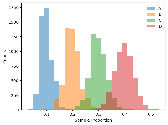
Figure 1: Sampling distribution of a multinomial distribution with four categories#
Notice how each of the four categories follow a binomial (approximately normal) sampling distribution.
This observation is going to be the eventual foundation of this project.
An (unsuccessful) simple attempt#
In the case of a one-proportion z-test, we can simulate the hypothesis test by creating a confidence interval from the sample proportion. If the given population proportion falls outside the interval, then we can conclude that there is evidence that the actual population proportion is different (or has changed). Specifically, a two-tailed z-test with significance level \(\alpha\) corresponds to a confidence interval with confidence level \((1 - \alpha)\).

Smahdavi4, CC BY-SA 4.0, via Wikimedia Commons
Important
Could we translate this analogy into the language of \(\chi^2\) tests?
Our very first obstacle is that the data are discrete counts, not proportions. This is easily fixed by dividing the counts by the sample size. After that, one potential way to approach this problem is to define the lower and upper limits of the interval for each category as the population proportion (for that category) with which it is just barely possible to avoid rejecting the null hypothesis with the given sample proportions.
However, this approach does not clearly answer the question stated in the first section:
I am XX% confident that the interval
____captures____.
since it does not guarantee that out of all possible samples of sample size \(n\), XX% of the corresponding confidence intervals would capture the true population proportion. Even if it were to do so, does every interval for every category capture the population proportion? What is the relationship across categories, as they’re clearly not independent?
If you’re interested in further investigating this method, Stan Brown has written an interesting article on it.
Adapting the one-proportion z-interval to \(\chi^2\) GOF tests#
Instead of attempting to reuse the relatively unfamiliar \(\chi^2\) distribution, let’s revert back to what we already know: the approximately normal sampling distribution created from binomial models.
For example, the following table shows a possible sample distribution as well as the corresponding 95% confidence z-interval for each of the four categories (sample size: 200).
Category |
Proportion |
Confidence Interval |
|---|---|---|
A |
0.075 |
(0.0385, 0.1115) |
B |
0.180 |
(0.1268, 0.2332) |
C |
0.370 |
(0.3031, 0.4369) |
D |
0.375 |
(0.3079, 0.4421) |
So now we can say,
I am 95% confident that the confidence interval (0.0385, 0.1115) captures the true population proportion for category A.
(and similar statements for the remaining categories)
Overall confidence level across multiple categories#
But what if we want to do more than giving a confidence interval for one category at a time only? Could we make the following statement:
I am XX% confident that each of the population proportions across all four categories lies within their respective confidence intervals.
We already have the intervals. They are listed in the table above. However, we do not know the confidence level. 95% is not the answer because that is the confidence level for one category only. The overall confidence level is certainly lower, since there is additional variance in the “not \(i\)th” category we mentioned earlier. The question is: how much lower?
The naive approach would be to multiply the confidence levels together (i.e. \(0.95^4\)), but that approach is incorrect because the assumption of independence is not met. In fact, the four sample proportions strictly abide by the following relationship:
It is a nontrivial task to utilize this relationship to mathematically determine how the variabilities for the four sample proportions affect one another. This project makes use of a computer-based simulation to experimentally determine the overall confidence level.
The simulation#
Simulation: The simulation consists of combinations of the following sample sizes and population proportions:
sample sizes \(n\)
50
100
200
500
1000
2000
population proportions \(p_i\) where \(1 \le i \le m\) and \(m\) is the number of categories
0.3, 0.7
0.1, 0.3, 0.6
0.2, 0.3, 0.5
0.25, 0.35, 0.4
\(\frac{1}{3}\), \(\frac{1}{3}\), \(\frac{1}{3}\)
0.1, 0.2, 0.3, 0.4
0.15, 0.25, 0.3, 0.3
0.25, 0.25, 0.25, 0.25
0.1, 0.1, 0.1, 0.1, 0.6
0.15, 0.15, 0.15, 0.15, 0.4
0.2, 0.2, 0.2, 0.2, 0.2
Combinations for which the success/failure condition (\(np \ge 10\)) isn’t met are excluded from the simulation.
Component: drawing a sample with sample size \(n\) and population proportions \(p_i\)
Outcome: The sample proportions are calculated by dividing counts by \(n\). One-proportion z-intervals at 95% confidence level are computed from each sample proportion. The number of categories for which the true population proportion falls within the confidence interval is determined.
Trials: 5000 trials are performed.
Response: The proportions of samples for which \(k\;(k \in \mathbb{Z}\cap [0, m])\) categories generate confidence intervals that capture their corresponding population proportions are recorded.
Simulation results#
A total of 20 simulations was performed for each combination of \(n\) and \(p_i\). The following table displays the mean and standard deviation of the 20 simulations for \(n = 100\) and \(p_i = \text{[0.15, 0.25, 0.3, 0.3]}\).
\(n\) |
\(p_i\) |
\(k\) |
0 |
1 |
2 |
3 |
4 |
|---|---|---|---|---|---|---|---|
100 |
[0.15, 0.25, 0.3, 0.3] |
\(\bar{x}_k\) |
0.00002 |
0.00143 |
0.0304 |
0.1543 |
0.81385 |
\(s_k\) |
\(6.2 \times 10^{-5}\) |
\(5.8 \times 10^{-4}\) |
\(2.5 \times 10^{-3}\) |
\(5.0 \times 10^{-3}\) |
\(5.0 \times 10^{-3}\) |
Tip
Full simulation results are available in Appendix A.
Observe how it is different from the binomial distribution \(\mathrm{Binom}(n = 4, p = 0.95, k)\) where independence between different trials (i.e. categories, in this scenario) is assumed.
\(k\) |
0 |
1 |
2 |
3 |
4 |
|---|---|---|---|---|---|
\(p\) |
0.00001 |
0.00047 |
0.01354 |
0.17147 |
0.81451 |
Now consider two other combinations of \(n\) and \(p_i\):
\(n\) |
\(p_i\) |
\(k = 0\) |
1 |
2 |
3 |
4 |
|---|---|---|---|---|---|---|
500 |
[0.15, 0.25, 0.3, 0.3] |
0.00012 |
0.00076 |
0.03316 |
0.14449 |
0.82147 |
100 |
[0.1, 0.2, 0.3, 0.4] |
0.00002 |
0.00175 |
0.03398 |
0.15838 |
0.80587 |
In the first row, \(n\) changed from 100 to 200. In the second row, \(n\) stayed the same, while \(p_i\) changed from [0.15, 0.25, 0.3, 0.3] to [0.1, 0.2, 0.3, 0.4]. For both rows, there are subtle changes in the mean for each value of \(k\). Are these differences significant?
Answering this question sounds exactly like the job of a hypothesis test.
Important
What type of test should be used?
Even though the data are proportions, the response variable itself (i.e. the confidence level we’re interested in, say, 82% or 0.82) can be considered quantitative in nature.
We ran each simulation 20 times, and we have means and standard deviations.
There are multiple (\(> 2\)) samples.
It seems that we need a variant of the two-mean t-test that generalizes to multiple means.
Performing a one-way ANOVA test#
One-way ANOVA tests detect differences between multiple means. ANOVA stands for ANalysis Of VAriance, and the test produces an F-statistic that is equal to the ratio of the variance between samples to the variance within the samples.
The P-value can then be calculated from using the F-distribution, which has two degree-of-freedom parameters.

IkamusumeFan, CC BY-SA 4.0, via Wikimedia Commons
Hypotheses#
\(H_0:\) The true population means of the overall confidence level that corresponds to a one-proportion z-interval at 95% confidence for each category of the multinomial distribution with \(p_i = [0.15, 0.25, 0.3, 0.3]\) are the same across different values of \(n\).
\(H_a:\) At least one of the aforementioned population means is different from the others.
Assumptions and conditions#
Independence: The data is generated using a pseudorandom generator with different seeds for each sample.
Population nearly normal: Histograms of sample distributions are nearly normal.
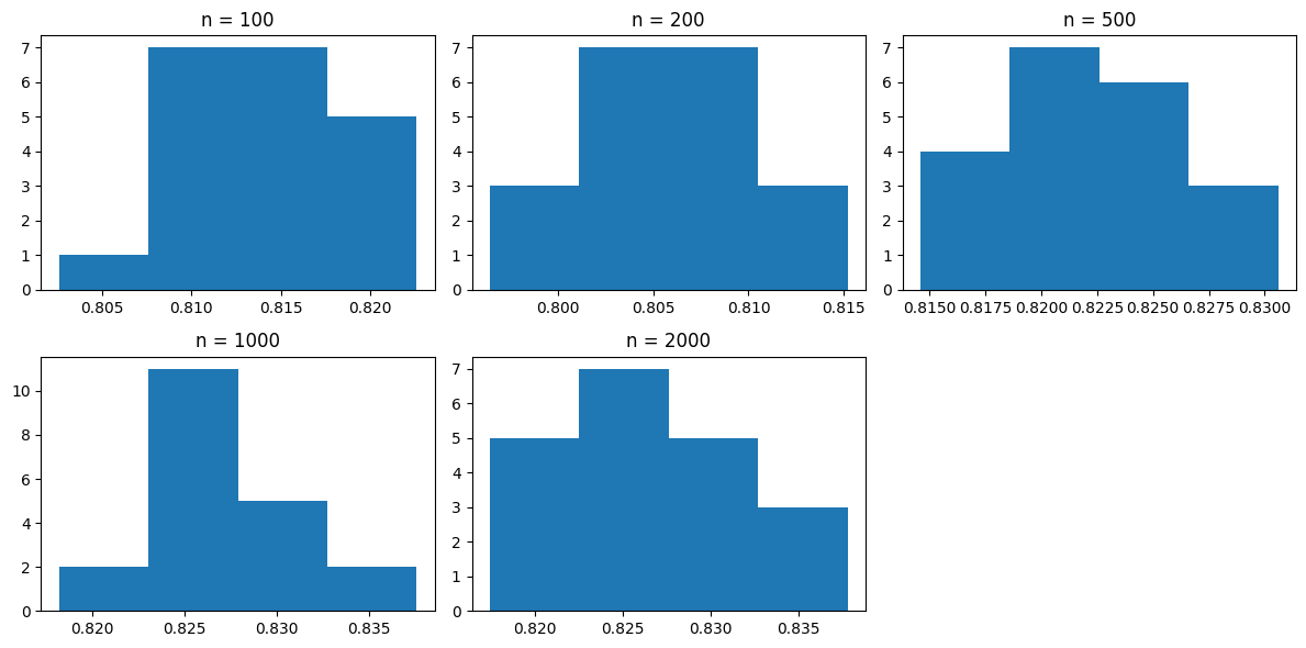
Figure 2: Histograms of sample distributions across multiple sample sizes#
Equal Variance: Sample standard deviations across different values of \(n\) are approximately equal.
\(n\)
\(s\)
100
\(5.0 \times 10^{-3}\)
200
\(5.1 \times 10^{-3}\)
500
\(4.7 \times 10^{-3}\)
1000
\(4.7 \times 10^{-3}\)
2000
\(5.7 \times 10^{-3}\)
Ok to perform a one-way ANOVA test at \(\mathrm{df1} = 4\), \(\mathrm{df2} = 95\), and \(\alpha = 0.05\)
F-statistic and P-value#
The scipy stats package gives
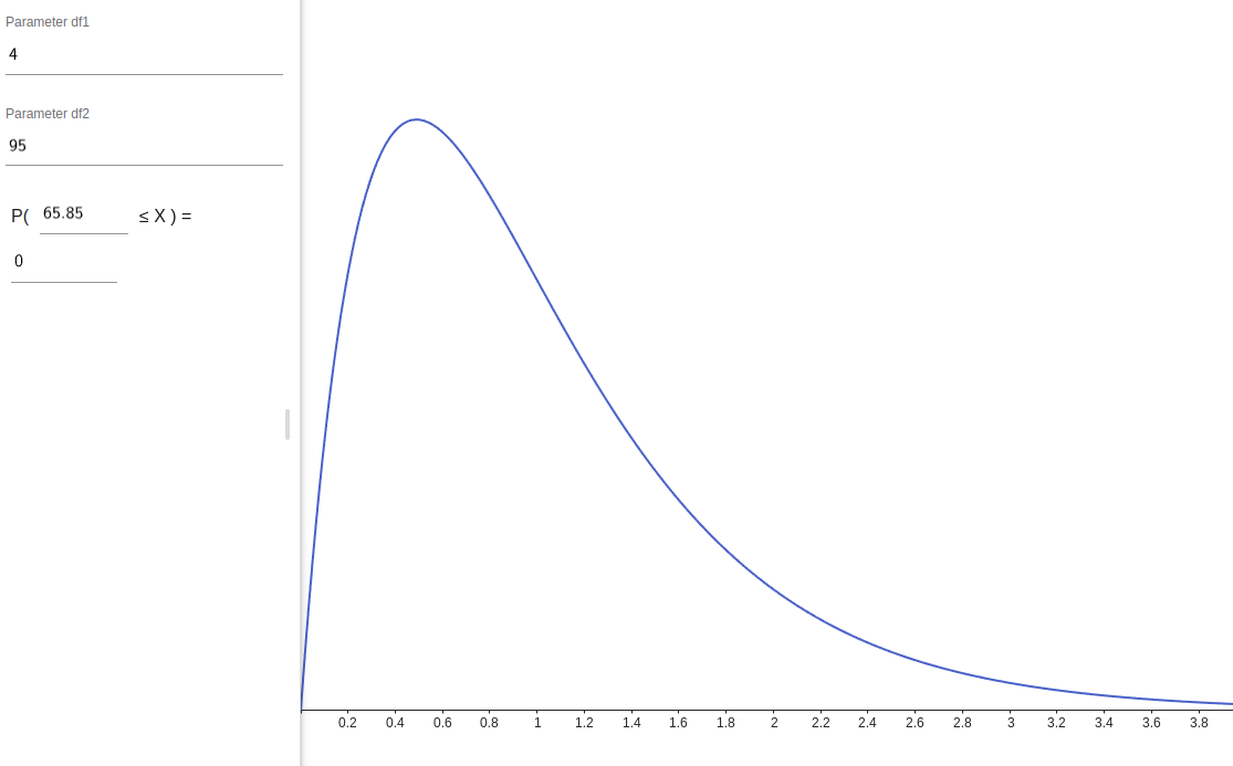
Figure 3: \(\chi^2\) distribution with \(\mathrm{df1} = 4\) and \(\mathrm{df2} = 95\)#
Conclusion#
The P-value is low, so I reject the null hypothesis. There is strong evidence that at least one of the true population means (across different values of \(n\)) of the overall confidence level that corresponds to a one-proportion z-interval at 95% confidence for each category of the multinomial distribution with \(p_i = [0.15, 0.25, 0.3, 0.3]\) is different from the others.
Similar tests are performed for other values of \(p_i\). A second set of one-way ANOVA tests are performed for each value of \(n\) across different values of \(p_i\). The null hypotheses are rejected in these tests.
Tip
Please refer to Appendix B for the full ANOVA test results.
Caution
The tests are also performed for each value of \(k\), i.e. the number of categories that generate confidence intervals that capture their corresponding population proportions. However, when \(k\) is small, assumptions for the one-way ANOVA test may be violated. Caution is required when interpreting these results.
Converting between individual and overall confidence levels#
Based on the previous section, we can conclude that the overall confidence level depends both on the sample size \(n\) and the population proportions \(p_i\). So how can we make use of this information to make a general statement about all categories?
If we are given a random sample, we already know the sample size. Obviously, we don’t know the population proportions, but we can reuse the same technique when we first studied confidence intervals: just pretend that the sample proportions are the population proportions! That’s how we came up with \(SE(\hat{p})\), right?
In other words, if we’re given a sample of size \(n\) and sample proportions \(\hat{p}_i\), we can temporarily assume that \(p_i = \hat{p}_i\) and rerun the simulation described in the previous section. The resulting proportion corresponding to \(k = m\) (reminder: \(m\) is the total number of categories) is therefore the overall confidence level across all categories.
Note that this procedure requires that we predetermine a confidence level for any individual category (i.e. the confidence level used in a one-proportion z-interval). What if we want to specify the overall confidence level instead?
In other words, if we want to make the following statement:
I am 90% confident that each of the population proportions across all four categories lies within their respective confidence intervals.
What confidence level should these “respective confidence intervals” (one-proportion z-intervals) use?
This problem can be solved by using a binary search for the individual confidence level. For example, if the target overall confidence level is 90%, let’s first assume that the corresponding individual confidence level is, say, 96%. Then we run the simulation and see if the resulting overall confidence level is less than or greater than the target value of 90%. After that, we can adjust our guess (96%) accordingly.
By repeating the procedure above, we are able to reach a close estimate of the true individual confidence level.
A Python implementation of this confidence-level conversion process can be found here.
Conclusion#
In this project, we investigated the multinomial distribution behind a \(\chi^2\) goodness-of-fit test. We executed a simulation to adapt the one-proportion z-interval to \(\chi^2\) GOF tests. We performed one-way ANOVA tests to determine whether the sample size and/or the population proportions had an impact on overall confidence level. Finally, we established a procedure of converting between individual and overall confidence levels.
This project allows us to confidently (hahaha) create confidence intervals for each of the categories of a multinomial distribution, and more importantly, to compute and interpret a confidence level that encapsulates the random variability across all categories.
Appendix A: Full simulation results#
\(n\) |
\(p_i\) |
\(k = 0\) |
1 |
2 |
3 |
4 |
5 |
|---|---|---|---|---|---|---|---|
50 |
[0.2, 0.2, 0.2, 0.2, 0.2] |
1e-05 |
7e-05 |
0.0038 |
0.03902 |
0.2204 |
0.7367 |
50 |
[0.2, 0.3, 0.5] |
0.00059 |
0.03973 |
0.1104 |
0.8493 |
||
50 |
[0.25, 0.25, 0.25, 0.25] |
4e-05 |
0.00186 |
0.0285 |
0.1731 |
0.7965 |
|
50 |
[0.25, 0.35, 0.4] |
0.00036 |
0.03306 |
0.1069 |
0.8597 |
||
50 |
[0.3, 0.7] |
0.0673 |
0 |
0.9327 |
|||
50 |
[\(\frac{1}{3}\), \(\frac{1}{3}\), \(\frac{1}{3}\)] |
0.00013 |
0.02843 |
0.09476 |
0.8767 |
||
100 |
[0.1, 0.1, 0.1, 0.1, 0.6] |
0 |
0.00026 |
0.00627 |
0.03904 |
0.2258 |
0.7287 |
100 |
[0.1, 0.2, 0.3, 0.4] |
2e-05 |
0.00175 |
0.03398 |
0.1584 |
0.8059 |
|
100 |
[0.1, 0.3, 0.6] |
0.00078 |
0.03131 |
0.09957 |
0.8683 |
||
100 |
[0.15, 0.15, 0.15, 0.15, 0.4] |
1e-05 |
0.0001 |
0.00484 |
0.04107 |
0.2247 |
0.7293 |
100 |
[0.15, 0.25, 0.3, 0.3] |
2e-05 |
0.00143 |
0.0304 |
0.1543 |
0.8139 |
|
100 |
[0.2, 0.2, 0.2, 0.2, 0.2] |
0 |
0.00019 |
0.00444 |
0.04926 |
0.2222 |
0.7239 |
100 |
[0.2, 0.3, 0.5] |
0.00035 |
0.034 |
0.1058 |
0.8598 |
||
100 |
[0.25, 0.25, 0.25, 0.25] |
4e-05 |
0.00105 |
0.02945 |
0.1547 |
0.8148 |
|
100 |
[0.25, 0.35, 0.4] |
8e-05 |
0.03067 |
0.1017 |
0.8676 |
||
100 |
[0.3, 0.7] |
0.05031 |
0 |
0.9497 |
|||
100 |
[\(\frac{1}{3}\), \(\frac{1}{3}\), \(\frac{1}{3}\)] |
4e-05 |
0.02322 |
0.08881 |
0.8879 |
||
200 |
[0.1, 0.1, 0.1, 0.1, 0.6] |
1e-05 |
0.00028 |
0.00649 |
0.04583 |
0.2288 |
0.7185 |
200 |
[0.1, 0.2, 0.3, 0.4] |
2e-05 |
0.00169 |
0.0353 |
0.1631 |
0.7999 |
|
200 |
[0.1, 0.3, 0.6] |
0.00105 |
0.03524 |
0.1064 |
0.8573 |
||
200 |
[0.15, 0.15, 0.15, 0.15, 0.4] |
1e-05 |
6e-05 |
0.00264 |
0.0371 |
0.1909 |
0.7692 |
200 |
[0.15, 0.25, 0.3, 0.3] |
3e-05 |
0.00124 |
0.03437 |
0.1585 |
0.8059 |
|
200 |
[0.2, 0.2, 0.2, 0.2, 0.2] |
1e-05 |
0.00013 |
0.00287 |
0.03777 |
0.2069 |
0.7523 |
200 |
[0.2, 0.3, 0.5] |
0.00025 |
0.03216 |
0.1042 |
0.8634 |
||
200 |
[0.25, 0.25, 0.25, 0.25] |
0.00014 |
0.0014 |
0.03941 |
0.1673 |
0.7917 |
|
200 |
[0.25, 0.35, 0.4] |
0.00011 |
0.03248 |
0.1043 |
0.8631 |
||
200 |
[0.3, 0.7] |
0.05589 |
0 |
0.9441 |
|||
200 |
[\(\frac{1}{3}\), \(\frac{1}{3}\), \(\frac{1}{3}\)] |
0.00014 |
0.02821 |
0.1001 |
0.8715 |
||
500 |
[0.1, 0.1, 0.1, 0.1, 0.6] |
0 |
0.0001 |
0.00367 |
0.03981 |
0.1896 |
0.7668 |
500 |
[0.1, 0.2, 0.3, 0.4] |
1e-05 |
0.00124 |
0.03231 |
0.1414 |
0.825 |
|
500 |
[0.1, 0.3, 0.6] |
0.00043 |
0.03229 |
0.09169 |
0.8756 |
||
500 |
[0.15, 0.15, 0.15, 0.15, 0.4] |
1e-05 |
0.00016 |
0.00235 |
0.03734 |
0.1785 |
0.7816 |
500 |
[0.15, 0.25, 0.3, 0.3] |
0.00012 |
0.00076 |
0.03316 |
0.1445 |
0.8215 |
|
500 |
[0.2, 0.2, 0.2, 0.2, 0.2] |
0 |
9e-05 |
0.00164 |
0.03661 |
0.1763 |
0.7854 |
500 |
[0.2, 0.3, 0.5] |
0.00017 |
0.03067 |
0.09411 |
0.8751 |
||
500 |
[0.25, 0.25, 0.25, 0.25] |
7e-05 |
0.00091 |
0.03624 |
0.1527 |
0.8101 |
|
500 |
[0.25, 0.35, 0.4] |
6e-05 |
0.02889 |
0.09887 |
0.8722 |
||
500 |
[0.3, 0.7] |
0.05092 |
0 |
0.9491 |
|||
500 |
[\(\frac{1}{3}\), \(\frac{1}{3}\), \(\frac{1}{3}\)] |
1e-05 |
0.0305 |
0.09667 |
0.8728 |
||
1000 |
[0.1, 0.1, 0.1, 0.1, 0.6] |
0 |
9e-05 |
0.00246 |
0.03406 |
0.1663 |
0.7971 |
1000 |
[0.1, 0.2, 0.3, 0.4] |
3e-05 |
0.00098 |
0.03199 |
0.1371 |
0.8299 |
|
1000 |
[0.1, 0.3, 0.6] |
0.00025 |
0.03123 |
0.08415 |
0.8844 |
||
1000 |
[0.15, 0.15, 0.15, 0.15, 0.4] |
0 |
0.00014 |
0.00225 |
0.03803 |
0.1835 |
0.7761 |
1000 |
[0.15, 0.25, 0.3, 0.3] |
5e-05 |
0.00066 |
0.03197 |
0.14 |
0.8274 |
|
1000 |
[0.2, 0.2, 0.2, 0.2, 0.2] |
0 |
0.00019 |
0.00179 |
0.0389 |
0.1828 |
0.7763 |
1000 |
[0.2, 0.3, 0.5] |
0.00016 |
0.03062 |
0.0957 |
0.8735 |
||
1000 |
[0.25, 0.25, 0.25, 0.25] |
6e-05 |
0.0006 |
0.03329 |
0.1461 |
0.8199 |
|
1000 |
[0.25, 0.35, 0.4] |
7e-05 |
0.02991 |
0.09679 |
0.8732 |
||
1000 |
[0.3, 0.7] |
0.04903 |
0 |
0.951 |
|||
1000 |
[\(\frac{1}{3}\), \(\frac{1}{3}\), \(\frac{1}{3}\)] |
4e-05 |
0.02625 |
0.09076 |
0.8829 |
||
2000 |
[0.1, 0.1, 0.1, 0.1, 0.6] |
1e-05 |
0.00015 |
0.00328 |
0.03826 |
0.1796 |
0.7787 |
2000 |
[0.1, 0.2, 0.3, 0.4] |
2e-05 |
0.00093 |
0.0312 |
0.1396 |
0.8282 |
|
2000 |
[0.1, 0.3, 0.6] |
0.00041 |
0.03335 |
0.08903 |
0.8772 |
||
2000 |
[0.15, 0.15, 0.15, 0.15, 0.4] |
1e-05 |
0.00015 |
0.00203 |
0.03743 |
0.1814 |
0.779 |
2000 |
[0.15, 0.25, 0.3, 0.3] |
2e-05 |
0.00072 |
0.03255 |
0.1399 |
0.8269 |
|
2000 |
[0.2, 0.2, 0.2, 0.2, 0.2] |
0 |
0.00017 |
0.0017 |
0.037 |
0.178 |
0.7831 |
2000 |
[0.2, 0.3, 0.5] |
0.00015 |
0.02877 |
0.09528 |
0.8758 |
||
2000 |
[0.25, 0.25, 0.25, 0.25] |
0.00011 |
0.00061 |
0.03239 |
0.145 |
0.8219 |
|
2000 |
[0.25, 0.35, 0.4] |
6e-05 |
0.02817 |
0.09321 |
0.8786 |
||
2000 |
[0.3, 0.7] |
0.05047 |
0 |
0.9495 |
|||
2000 |
[\(\frac{1}{3}\), \(\frac{1}{3}\), \(\frac{1}{3}\)] |
7e-05 |
0.0278 |
0.09806 |
0.8741 |
\(n\) |
\(p_i\) |
\(k = 0\) |
1 |
2 |
3 |
4 |
5 |
|---|---|---|---|---|---|---|---|
50 |
[0.2, 0.2, 0.2, 0.2, 0.2] |
4.472e-05 |
0.0001174 |
0.001114 |
0.001677 |
0.004869 |
0.004965 |
50 |
[0.2, 0.3, 0.5] |
0.0002469 |
0.002966 |
0.005519 |
0.006237 |
||
50 |
[0.25, 0.25, 0.25, 0.25] |
8.208e-05 |
0.0006524 |
0.001837 |
0.005336 |
0.005783 |
|
50 |
[0.25, 0.35, 0.4] |
0.000201 |
0.002136 |
0.003811 |
0.004924 |
||
50 |
[0.3, 0.7] |
0.003095 |
0 |
0.003095 |
|||
50 |
[\(\frac{1}{3}\), \(\frac{1}{3}\), \(\frac{1}{3}\)] |
0.0001342 |
0.002093 |
0.004222 |
0.004812 |
||
100 |
[0.1, 0.1, 0.1, 0.1, 0.6] |
0 |
0.0001847 |
0.0009825 |
0.00301 |
0.004722 |
0.005744 |
100 |
[0.1, 0.2, 0.3, 0.4] |
6.156e-05 |
0.0007104 |
0.003224 |
0.005613 |
0.006659 |
|
100 |
[0.1, 0.3, 0.6] |
0.0003778 |
0.002558 |
0.004149 |
0.004752 |
||
100 |
[0.15, 0.15, 0.15, 0.15, 0.4] |
4.472e-05 |
0.0001654 |
0.0007937 |
0.003357 |
0.006717 |
0.00614 |
100 |
[0.15, 0.25, 0.3, 0.3] |
6.156e-05 |
0.0005777 |
0.002503 |
0.005012 |
0.005019 |
|
100 |
[0.2, 0.2, 0.2, 0.2, 0.2] |
0 |
0.0001651 |
0.0008375 |
0.002285 |
0.00394 |
0.003973 |
100 |
[0.2, 0.3, 0.5] |
0.0002236 |
0.00175 |
0.005543 |
0.005165 |
||
100 |
[0.25, 0.25, 0.25, 0.25] |
8.208e-05 |
0.0004807 |
0.001973 |
0.004973 |
0.004863 |
|
100 |
[0.25, 0.35, 0.4] |
0.0001005 |
0.002463 |
0.004322 |
0.005227 |
||
100 |
[0.3, 0.7] |
0.002522 |
0 |
0.002522 |
|||
100 |
[\(\frac{1}{3}\), \(\frac{1}{3}\), \(\frac{1}{3}\)] |
8.208e-05 |
0.002137 |
0.004574 |
0.005125 |
||
200 |
[0.1, 0.1, 0.1, 0.1, 0.6] |
4.472e-05 |
0.0002285 |
0.001329 |
0.002614 |
0.005923 |
0.006105 |
200 |
[0.1, 0.2, 0.3, 0.4] |
6.156e-05 |
0.000788 |
0.003207 |
0.005785 |
0.006398 |
|
200 |
[0.1, 0.3, 0.6] |
0.0003103 |
0.002492 |
0.004847 |
0.005532 |
||
200 |
[0.15, 0.15, 0.15, 0.15, 0.4] |
4.472e-05 |
9.403e-05 |
0.0006855 |
0.002834 |
0.005291 |
0.006083 |
200 |
[0.15, 0.25, 0.3, 0.3] |
7.327e-05 |
0.0003705 |
0.002561 |
0.004643 |
0.005143 |
|
200 |
[0.2, 0.2, 0.2, 0.2, 0.2] |
4.472e-05 |
0.0001625 |
0.0007767 |
0.002302 |
0.005942 |
0.006568 |
200 |
[0.2, 0.3, 0.5] |
0.0002236 |
0.00254 |
0.003515 |
0.003984 |
||
200 |
[0.25, 0.25, 0.25, 0.25] |
0.0001465 |
0.0006358 |
0.00318 |
0.005248 |
0.005454 |
|
200 |
[0.25, 0.35, 0.4] |
0.000121 |
0.001857 |
0.004097 |
0.003811 |
||
200 |
[0.3, 0.7] |
0.002599 |
0 |
0.002599 |
|||
200 |
[\(\frac{1}{3}\), \(\frac{1}{3}\), \(\frac{1}{3}\)] |
0.0001603 |
0.002422 |
0.005318 |
0.005824 |
||
500 |
[0.1, 0.1, 0.1, 0.1, 0.6] |
0 |
0.0001214 |
0.0009782 |
0.002535 |
0.003902 |
0.004516 |
500 |
[0.1, 0.2, 0.3, 0.4] |
4.472e-05 |
0.0005335 |
0.002277 |
0.005515 |
0.005739 |
|
500 |
[0.1, 0.3, 0.6] |
0.0002179 |
0.001736 |
0.005173 |
0.005372 |
||
500 |
[0.15, 0.15, 0.15, 0.15, 0.4] |
4.472e-05 |
0.0001536 |
0.0008457 |
0.002234 |
0.00505 |
0.005098 |
500 |
[0.15, 0.25, 0.3, 0.3] |
0.0001508 |
0.0003016 |
0.002471 |
0.004079 |
0.004686 |
|
500 |
[0.2, 0.2, 0.2, 0.2, 0.2] |
0 |
0.0001373 |
0.0006636 |
0.002471 |
0.007213 |
0.007644 |
500 |
[0.2, 0.3, 0.5] |
0.0001625 |
0.002638 |
0.004529 |
0.004641 |
||
500 |
[0.25, 0.25, 0.25, 0.25] |
0.0001174 |
0.0004564 |
0.002482 |
0.005682 |
0.004796 |
|
500 |
[0.25, 0.35, 0.4] |
9.403e-05 |
0.001542 |
0.003913 |
0.004057 |
||
500 |
[0.3, 0.7] |
0.002424 |
0 |
0.002424 |
|||
500 |
[\(\frac{1}{3}\), \(\frac{1}{3}\), \(\frac{1}{3}\)] |
4.472e-05 |
0.002093 |
0.004628 |
0.005638 |
||
1000 |
[0.1, 0.1, 0.1, 0.1, 0.6] |
0 |
0.000121 |
0.0006589 |
0.001899 |
0.006254 |
0.005838 |
1000 |
[0.1, 0.2, 0.3, 0.4] |
7.327e-05 |
0.0004396 |
0.001997 |
0.006037 |
0.005956 |
|
1000 |
[0.1, 0.3, 0.6] |
0.0002236 |
0.002591 |
0.004201 |
0.00462 |
||
1000 |
[0.15, 0.15, 0.15, 0.15, 0.4] |
0 |
0.0001957 |
0.0007015 |
0.003165 |
0.004343 |
0.004244 |
1000 |
[0.15, 0.25, 0.3, 0.3] |
8.885e-05 |
0.0003619 |
0.002626 |
0.004584 |
0.004668 |
|
1000 |
[0.2, 0.2, 0.2, 0.2, 0.2] |
0 |
0.00021 |
0.0006973 |
0.002645 |
0.005072 |
0.004926 |
1000 |
[0.2, 0.3, 0.5] |
0.0001789 |
0.002666 |
0.004127 |
0.005031 |
||
1000 |
[0.25, 0.25, 0.25, 0.25] |
0.0001142 |
0.0003554 |
0.002571 |
0.005882 |
0.005955 |
|
1000 |
[0.25, 0.35, 0.4] |
9.787e-05 |
0.002482 |
0.004317 |
0.005576 |
||
1000 |
[0.3, 0.7] |
0.002381 |
0 |
0.002381 |
|||
1000 |
[\(\frac{1}{3}\), \(\frac{1}{3}\), \(\frac{1}{3}\)] |
0.0001046 |
0.002361 |
0.004158 |
0.004199 |
||
2000 |
[0.1, 0.1, 0.1, 0.1, 0.6] |
4.472e-05 |
0.0002417 |
0.001004 |
0.002584 |
0.005203 |
0.006214 |
2000 |
[0.1, 0.2, 0.3, 0.4] |
6.156e-05 |
0.0004601 |
0.001785 |
0.007363 |
0.007378 |
|
2000 |
[0.1, 0.3, 0.6] |
0.0002936 |
0.003295 |
0.004425 |
0.005209 |
||
2000 |
[0.15, 0.15, 0.15, 0.15, 0.4] |
4.472e-05 |
0.0001701 |
0.0006689 |
0.002727 |
0.00641 |
0.005586 |
2000 |
[0.15, 0.25, 0.3, 0.3] |
6.156e-05 |
0.0003071 |
0.002536 |
0.006051 |
0.00566 |
|
2000 |
[0.2, 0.2, 0.2, 0.2, 0.2] |
0 |
0.0002179 |
0.0006308 |
0.002828 |
0.006652 |
0.006575 |
2000 |
[0.2, 0.3, 0.5] |
0.0002328 |
0.002497 |
0.004365 |
0.004656 |
||
2000 |
[0.25, 0.25, 0.25, 0.25] |
0.0001373 |
0.0003076 |
0.001785 |
0.004795 |
0.005171 |
|
2000 |
[0.25, 0.35, 0.4] |
0.0001142 |
0.002132 |
0.004306 |
0.005106 |
||
2000 |
[0.3, 0.7] |
0.003421 |
0 |
0.003421 |
|||
2000 |
[\(\frac{1}{3}\), \(\frac{1}{3}\), \(\frac{1}{3}\)] |
0.0001342 |
0.002582 |
0.004185 |
0.004475 |
Appendix B: Full one-way ANOVA test results#
\(p_i\) |
\(k = 0\) |
1 |
2 |
3 |
4 |
5 |
|---|---|---|---|---|---|---|
[0.1, 0.1, 0.1, 0.1, 0.6] |
0.75 |
4.555 |
65.34 |
54.79 |
565.5 |
681.8 |
[0.1, 0.2, 0.3, 0.4] |
0.2669 |
8.207 |
8.306 |
76.33 |
92.54 |
|
[0.1, 0.3, 0.6] |
24.9 |
8.35 |
74.32 |
80.46 |
||
[0.15, 0.15, 0.15, 0.15, 0.4] |
0.25 |
1.354 |
47.94 |
6.472 |
226.5 |
311.5 |
[0.15, 0.25, 0.3, 0.3] |
4.062 |
15.46 |
6.686 |
60.06 |
65.85 |
|
[0.2, 0.2, 0.2, 0.2, 0.2] |
0.8 |
1.808 |
44.75 |
78.78 |
276.9 |
383.4 |
[0.2, 0.3, 0.5] |
12.75 |
46.79 |
42.38 |
89.34 |
||
[0.25, 0.25, 0.25, 0.25] |
2.421 |
19.19 |
60.92 |
91.28 |
107.8 |
|
[0.25, 0.35, 0.4] |
17.12 |
16.67 |
29.45 |
41.66 |
||
[0.3, 0.7] |
125.8 |
125.8 |
||||
[\(\frac{1}{3}\), \(\frac{1}{3}\), \(\frac{1}{3}\)] |
4.095 |
23.12 |
18.44 |
32.74 |
\(p_i\) |
\(k = 0\) |
1 |
2 |
3 |
4 |
5 |
|---|---|---|---|---|---|---|
[0.1, 0.1, 0.1, 0.1, 0.6] |
0.5604 |
0.002077 |
1.909e-26 |
7.245e-24 |
2.646e-65 |
5.113e-69 |
[0.1, 0.2, 0.3, 0.4] |
0.8986 |
9.953e-06 |
8.653e-06 |
7.922e-29 |
6.588e-32 |
|
[0.1, 0.3, 0.6] |
4.065e-14 |
8.137e-06 |
2.066e-28 |
1.172e-29 |
||
[0.15, 0.15, 0.15, 0.15, 0.4] |
0.909 |
0.2559 |
5.298e-22 |
0.0001193 |
1.151e-47 |
1.1e-53 |
[0.15, 0.25, 0.3, 0.3] |
0.004395 |
8.957e-10 |
8.739e-05 |
3.405e-25 |
1.465e-26 |
|
[0.2, 0.2, 0.2, 0.2, 0.2] |
0.5519 |
0.1168 |
2.38e-25 |
2.373e-35 |
5.081e-62 |
1.545e-69 |
[0.2, 0.3, 0.5] |
7.654e-10 |
4.452e-26 |
1.773e-24 |
8.829e-38 |
||
[0.25, 0.25, 0.25, 0.25] |
0.03986 |
8.148e-14 |
1.324e-30 |
3.343e-38 |
1.574e-41 |
|
[0.25, 0.35, 0.4] |
1.323e-12 |
2.472e-12 |
4.296e-19 |
3.313e-24 |
||
[0.3, 0.7] |
1.05e-44 |
1.05e-44 |
||||
[\(\frac{1}{3}\), \(\frac{1}{3}\), \(\frac{1}{3}\)] |
0.001863 |
5.715e-16 |
2.193e-13 |
1.404e-20 |
\(n\) |
\(m\) |
\(k = 0\) |
1 |
2 |
3 |
4 |
5 |
|---|---|---|---|---|---|---|---|
50 |
3 |
26.59 |
109.2 |
64.1 |
132.8 |
||
100 |
3 |
44.31 |
84.29 |
48.11 |
111.6 |
||
100 |
4 |
0.5588 |
6.889 |
16.66 |
3.73 |
15.4 |
|
100 |
5 |
1 |
4.35 |
24.18 |
68.74 |
2.469 |
5.9 |
200 |
3 |
85.17 |
30.47 |
6.78 |
28.7 |
||
200 |
4 |
8.684 |
2.686 |
16.01 |
14.24 |
31.2 |
|
200 |
5 |
3.444e-33 |
8.665 |
98.54 |
70.24 |
220.9 |
340.7 |
500 |
3 |
33.13 |
9.235 |
9.227 |
2.244 |
||
500 |
4 |
4.724 |
6.196 |
14.7 |
25.45 |
46.56 |
|
500 |
5 |
1 |
1.505 |
30.14 |
9.629 |
32.93 |
55.16 |
1000 |
3 |
7.023 |
15.63 |
37.66 |
29.87 |
||
1000 |
4 |
0.532 |
5.558 |
1.962 |
13.94 |
17.47 |
|
1000 |
5 |
1.546 |
4.989 |
19.37 |
68.17 |
114.6 |
|
2000 |
3 |
12.45 |
18.85 |
15.5 |
3.122 |
||
2000 |
4 |
6.131 |
3.959 |
2.55 |
4.841 |
5.858 |
|
2000 |
5 |
0.5 |
0.05933 |
22.49 |
1.113 |
1.565 |
3.247 |
\(n\) |
\(m\) |
\(k = 0\) |
1 |
2 |
3 |
4 |
5 |
|---|---|---|---|---|---|---|---|
50 |
3 |
6.959e-09 |
3.217e-20 |
2.601e-15 |
3.534e-22 |
||
100 |
3 |
1.152e-16 |
4.119e-24 |
1.557e-17 |
9.056e-28 |
||
100 |
4 |
0.575 |
0.002091 |
2.006e-06 |
0.03004 |
4.486e-06 |
|
100 |
5 |
0.3742 |
0.01745 |
2.488e-08 |
6.456e-16 |
0.09371 |
0.004688 |
200 |
3 |
3.047e-24 |
4.857e-13 |
0.0004118 |
1.632e-12 |
||
200 |
4 |
0.0005105 |
0.07679 |
3.029e-06 |
9.624e-06 |
7.055e-10 |
|
200 |
5 |
1 |
0.0005177 |
3.166e-19 |
4.175e-16 |
1.411e-27 |
1.98e-32 |
500 |
3 |
8.437e-14 |
2.786e-05 |
2.811e-05 |
0.08992 |
||
500 |
4 |
0.01264 |
0.003673 |
7.108e-06 |
1.262e-08 |
1.031e-12 |
|
500 |
5 |
0.3742 |
0.2308 |
1.174e-09 |
0.0002497 |
3.119e-10 |
4.694e-14 |
1000 |
3 |
0.0003132 |
5.198e-08 |
5.085e-15 |
7.299e-13 |
||
1000 |
4 |
0.5903 |
0.006235 |
0.1499 |
1.177e-05 |
1.208e-06 |
|
1000 |
5 |
0.222 |
0.01008 |
3.807e-07 |
7.635e-16 |
1.057e-20 |
|
2000 |
3 |
1.043e-06 |
3.076e-09 |
5.863e-08 |
0.03081 |
||
2000 |
4 |
0.003874 |
0.02455 |
0.08697 |
0.01143 |
0.004855 |
|
2000 |
5 |
0.6092 |
0.9425 |
6.314e-08 |
0.3356 |
0.218 |
0.04619 |
This article is licensed under CC BY-SA 4.0.