Physics#
Motion#
In an \(O-xyz\) coordinate system the position vector \(\vec r\) is defined as:
Its magnitude is:
In polar coordinates, it is usually defined in terms of \(r\) and \(\theta\).
The displacement vector \(\Delta\vec s\) is defined as:
The average velocity is:
The instantaneous velocity and acceleration is:
Formulas for constant acceleration motion on a straight line:
Strategy: Maximum/minimum values
write down the expression for the variable
simplify the expression so that it contains one and only one independent variable
mathematically determine the extremum
Alternative strategy: Maximum/minimum values
This is best suited for geometric problems (instead of ones that requires tons of calculation).
try to determine the position of extremum by intuition (sort of obscure)
rigorously prove your intuition
solve the problem
General motion in polar coordinates:
Projectile motion#
Model: Falling objects with initial upward velocity
Model: Objects falling onto a tilted surface
create a coordinate system with the surface as the x(y)-axis
identify the initial conditions (velocity, position and acceleration)
plug in the equations and solve the problem
Circular and spiral motion#
Rigid bodies:
translational motion
rotational motion
combination motion
Angular velocity
Angular acceleration
Constant-angular-acceleration rotational motion:
The radius of curvature \(\rho\):
Tip
The acceleration of an object stays the same in different inertial reference frames.
Tip
Switching inertial reference frames is an excellent way to calculate acceleration.
Example
if the center of rotation is stationary in a particular reference frame
Strategy: Problems involving the angle between two vector quantities
Express the vector (for example, velocity or acceleration) by selecting a pair of basis vectors and then utilizing the dot product:
Or more specifically, when \(\vec{u}\perp\vec{v}\),
Note
A reference frame can be rotating, in which case it is called a rotating reference frame. A rotating reference frame is not an inertial reference frame.
If a rotating object seems to be stationary in a rotating reference frame, then it has the same angular speed as the rotating frame itself, although the direction of \(\omega\) (angular velocity) is reversed.
Tip
When the relative motion between two objects is involved and one of the objects has a fixed velocity and/or acceleration, try switching reference frames.
The balance of objects#
The balance of forces#
Types of forces:
gravitational force
elastic force
friction
\(\dots\)
Springs:
where \(k\) is the spring constant.
Multiple springs:
series:
\[ \frac{1}{k} = \frac{1}{k_1} + \frac{1}{k_2} + \cdots \]parallel:
\[ k = k_1 + k_2 + \cdots \]
Friction angle:
let \(\mu = \tan\varphi\), then
Generally, \(f_{static} < f_{max}\). Therefore,
The angle \(\alpha\) between the full reaction force \(F\) and the normal line cannot be greater than the friction angle \(\varphi\)
Attention
When the solution to a problem can not be specified as a fixed value, solve for the range of values it lies in.
Strategy: Balancing objects influenced by friction
use “friction angles”
\[ \tan\varphi = \mu \]use geometry and trigonometry to figure out the relationship between the angles
substitute \(\mu\) back in and get the answer
Strategy: The fewer forces, the better
When a large object is in balance, try to find a segment of the object on which the fewest forces act. In other words, restrict yourself to one or two forces.
Young’s modulus
Shear modulus
Moment and rotation#
Condition for balance:
Force couples:
where \(\tau\) is the torque the couple has on the object and \(d\) is the distance between the two forces.
The synthesis of parallel forces
Let \(|AO|\) be the distance between \(F\) (the combined force) and \(F_1\), and \(|BO|\) be the distance between \(F\) and \(F_2\), then
The magnitude of \(F\) depends on whether \(F_1\) and \(F_2\) are in the same direction or not.
Model: An object with a hole in it
pretend that the hole doesn’t exist
recreate the hole by putting a force in the opposite direction
Tip
If the direction of a force is unknown, suppose it is in a specific direction and determine whether the system can stay in balance.
Alternatively, use a coordinate system, write down the force as a general vector \(x\hat i + y\hat j + z\hat k\) and apply linear algebra
Model: Steelyard balance
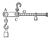
(By An Elementary Treatise on Analytic Mechanics: With Numerous Examples By Edward A. (Edward Albert) Bowser, 1893., Public Domain, Link)
Let \(|AC| = d\), \(|CO| = l_0\), and let \(M\) be the moment the gravity of the whole balance has on the pivot \(C\)
Then if the mass of the weight is \(m\), and the mass of the counterweight is \(m_0\), we have
and
where \(\lambda\) is the ratio of the distance between \(O\) and the counterweight and \(m\).
Therefore,
This is the fundamental equation of steelyard balances.
Tip
A useful trigonometric identity (half angle formula for \(\tan\)):
Important
When the number of equations is smaller than the unknowns, the system is statically indeterminate. Look for hidden details in the text.
Tip
Focal radii for ellipse
where \(a \ge b > 0\):
Let \(F_1\) denote the left focus and \(F_2\) denote the right focus, and let \(P(m, n)\) be a point on the ellipse, then
Liquids in static equilibrium#
Important
Bernoulli’s principle:
Note
Centrifugal potential energy:
Newton’s laws#
first: inertia
second: \(F = ma\)
third: action and reaction
Note
Newton’s laws only apply under macroscopic, low-speed conditions.
Acceleration is the bridge between force and motion.
Strategy: How to find acceleration
relative motion
\[ a_{abs} = a_{sys} + a_{rel} \]-
\[ \lim_{t \to 0}\frac{s_1(t)}{s_2(t)} = \lim_{t \to 0}\frac{v_1(t)}{v_2(t)} = \lim_{t \to 0}\frac{a_1(t)}{a_2(t)} \]
provided that when \(t \to 0\), both \(v_1\) and \(v_2\) \(\to 0\).
Touching objects have the same acceleration in the direction of the line perpendicular to the surface
Non-inertial reference frames#
Inertial force
Rotating reference frames:
Planetary motion#
Kepler’s laws:
first
second
third:
\[ \frac{T^2}{a^3} = \frac{4\pi^2}{GM} \]
Newton’s law of gravity:
where \(G=6.67\times 10^{-11} N\cdot m^2/kg^2\)
Tip
To avoid using the gravitational constant or the mass of the Sun/Earth, find the ratio between the unknown quantitiy and what we already know.
Important
Momentum and angular momentum#
Impluse
The impulse-momentum theorem:
Variable-mass system:
For rockets:
Moment of inertia:
The parallel axis theorem:
The perpendicular axis theorem:
If a flat disk is in the \(xy\)-plane, then
Object |
Moment of inertia |
|---|---|
rod/slab |
\(\frac{1}{12}mL^2\) or \(\frac{1}{3}mL^2\) |
cylinder/disk |
\(\frac{1}{2}mR^2\) |
hoop |
\(mR^2\) |
sphere |
\(\frac{2}{5}mR^2\) |
spherical shell |
\(\frac{2}{3}mR^2\) |
Angular momentum:
The formula
is only true when rotating about an axis of symmetry or a fixed axle.
Energy#
Work and Power#
Work
Power
Important
Energy and work are frame-dependent!
Work and Energy#
The work-kinetic energy theorem:
Conservation of mechanical energy:
where \(K\) and \(U\) are kinetic energy and potential energy, respectively.
Collisions#
During a perfectly inelastic collision, the two objects move together and only momentum is conserved.
During a perfectly elastic collision, both momentum and energy are conserved:
- Coefficient of restitution
the ratio of the relative speed after and before the collision
For a perfectly elastic collision, \(e = 1\).
For a perfectly inelastic collision, \(e = 0\).
Otherwise, \(0 < e < 1\).
Satellite orbits and energies#
Strategy
Kepler’s second law or conservation of angular momentum
\[ rv\sin\alpha = r'v'\sin\beta \]where \(\alpha\) and \(\beta\) are the angle between \(\mathbf{r}\) and \(\mathbf{v}\).
Conservation of energy
\[ E = E_k + E_{grav} = E_k' + E_{grav}' \]Orbit type
\(E\)
Ellipse
\(-\frac{GMm}{2a}\)
Parabola
\(0\)
Hyperbola
\(\frac{GMm}{2a}\)
Tip
Useful trigonometric identities:
Reverse identities:
Caution
Be careful with the ranges of the inverse trigonometric functions!
Function |
Range |
|---|---|
\(\arcsin x\) |
\([-\frac{\pi}{2}, \frac{\pi}{2}]\) |
\(\arccos x\) |
\([0, \pi]\) |
\(\arctan x\) |
\((-\frac{\pi}{2}, \frac{\pi}{2})\) |
Oscillations and waves#
Simple harmonic motion#
Position, speed and acceleration:
For a second-order differential equation in the form
the solution is simply SHM with angular frequency \(\omega\).
Period:
For springs and simple pendulums,
Strategy: General SHM
In more general conditions other than springs and pendulums, try to determine the system’s equivalent “mass” and “spring coefficient”.
write down the system’s potential energy \(V(q)\) where \(q\) is a custom variable
The equilibrium points are those such that \(V'(q) = 0\).
The equivalent “spring coefficient” \(k^*\) is given by \(V''(q)\)
determine the equivalent “mass” by writing down the kinetic energy:
\[ T(\dot{q}) = \frac{1}{2}m^*\dot{q}^2 \]plug everything into the spring equation above
Waves#
A sinusoidal wave
has the following properties:
Name |
Value |
|---|---|
amplitude |
\(A\) |
frequency |
\(f\) |
wavelength |
\(\lambda\) |
initial phase |
\(\varphi_0\) |
angular frequency |
\(\omega = 2\pi f = \frac{2\pi}{T}\) |
period |
\(T = \frac{1}{f} = \frac{2\pi}{\omega}\) |
wave number |
\(k = \frac{2\pi}{\lambda}\) |
wave speed |
\(v = \lambda f = \frac{\lambda}{T}\) |
phase |
\(\varphi = \varphi_0 + \omega t\) |
Note
It is perfectly fine (although highly discouraged, see the note below) to replace the cosine function with a sine function, however do keep in mind the differences between sine and cosine, including the ranges of their inverse functions (see above).
In the wave equation above, if \(x\) is fixed at \(x_0\), then \(y\) turns into a function of \(t\). This function represents the oscillation at a fixed point as time goes on.
There is a subtle but extremely important detail in the equation above, namely the fact that the actual phase is represented by \(\varphi_0 + \omega t\), while the term \(-kx\) determines the displacement at different x-coordinates.
As a result, if the wave travels in the opposite direction, the signs of both \(\varphi_0\) and \(\omega t\) need to be inverted. However, as the cosine function is an even function, it is equivalent with replacing \(-kx\) with \(kx\). (If a sine function is used instead, make sure that an additional minus sign is added.)
Tip
For both sine and cosine functions, if \(kx\) and \(\omega t\) are opposite in sign, the wave travels to the right. If they are the same in sign, the wave travels to the left.
Important
In simple problems concerning waves (especially the phases of a travelling wave), it is highly recommended to stick to the cosine expression above. The reason is that at a fixed point, it is not at all intuitive to have a \(-\omega t\) term, as if the “phase” is “decreasing”, like this:
(even though I have seen many books and websites recommend this approach)
Therefore, in more complex problems, it is usually much more preferable to use complex exponentials so as to avoid the tricky phase problem.
Waves as complex exponentials#
where
is the complex amplitude.
The complex conjugate of the wave function is
To transform the complex wave function back into a trigonometric one, simply apply this formula:
Warning
In the second equation, as the wave travels to the right, there is a \(-kx\) term in the \(\sin\), which is an odd function. As a result, the phase of the wave is also “inverted”.
Therefore, under most circumstances, it definitely should NOT be used.
According to a rule concerning complex conjugates, we have
Standing waves#
When two waves have the same amplitude, frequency and wavelength and at the same time travels in the opposite direction, they interfere with each other and produce a standing wave.
The amplitude function
Tip
Euler’s formula:
For tubes/strings, there are three distinct cases
Type |
Endpoint |
Frequency |
|---|---|---|
closed-closed |
node |
\(f = n\frac{v}{2L}\) |
open-open |
antinode |
\(f = n\frac{v}{2L}\) |
open-closed |
mixed |
\(f = (n - \frac{1}{2})\frac{v}{2L}\) |
The Doppler effect#
In the table below, the velocities of the source, the observer and the wave in the medium are \(u\), \(v\) and \(c\), respectively.
Source |
Observer |
Frequency |
|---|---|---|
stationary |
stationary |
\(f' = f\) |
stationary |
moving |
\(f' = \frac{c \pm v}{c}f\) |
moving |
stationary |
\(f' = \frac{c}{c \mp u}f\) |
moving |
moving |
\(f' = \frac{c \pm v}{c \mp u}f\) |
Note
When both the source and the observer are moving, it is not recommended to use the equation above as it may yield incorrect answers when the velocities are not on the same line.
Instead, trace the motion of a single wave crest (or trough) and use the definition of the frequency.
Alternatively, use this formula:
where \(\alpha\) and \(\beta\) are the angles between the velocities and the line connecting the source and the observer.
Important
The velocity of a wave (\(v = \lambda f\)) is the velocity relative to the medium!
Thermodynamics#
The ideal gas law#
Avogrado’s number
Boltzmann’s constant
Let \(n\) be the particle density \(N/V\), and we get
By analyzing the motion of each molecule and adding them all together, we get
Combining the last two equations together, here is another formula for \(\overline{E_k}\):
Tip
The binomial approximation:
Tip
The first law of thermodynamics#
The change in internal energy equals the sum of the heat transferred from the environment and the work done by the environment.
Caution
Make sure the signs before \(Q\) and \(W\) are correct! They must correspond to the heat FROM the environment and the work BY the environment!
The work done on the system can always be calculated with integration:
Caution
When calculating the work, never ever forget to take the atmospheric pressure \(p_0\) into account.
Ideal-gas processes#
Isochoric (constant-volume)
Isobaric (constant-pressure)
Isothermal (constant-temperature)
Adiabatic
If
then we have
Strategy: Multistep processes
If a process involves more than two states, such as this one:
then directly analyzing \(A \to B\) and \(B \to C\) may not be plausible.
Instead, try \(A \to C\).
Surface phenomena#
Surface tension is caused by the attractive forces between molecules of a liquid.
Alternatively, use the work-area formula:
Wetting and capillary action depends on the cohesion between liquid molecules and the adhesion among liquid and solid molecules.
Let \(\theta\) be the contact angle, and \(r\) be the radius of the tube, then
Therefore
Laplace pressure
where \(\rho_x\) and \(\rho_y\) are the radii of curvature in two perpendicular directions parallel to the surface.
Proof:
Important
Laplace pressure is very useful, especially when one of the radii (or both of them) is \(\infty\).
Heat transfer and thermal expansion#
Conduction
Radiation (black body)
Radiation
Note
Concerning thermal expansion, I have seen various different expressions contradicting one another.
Therefore, this topic is currently omitted.
Maxwell-Boltzmann distribution#
There are three distinct speeds related to this distribution
The average speed
The root-mean-square speed
The most probable speed
The second law of thermodynamics#
The entropy of an isolated system never decreases.
Heat cannot be spontaneously transferred from a cold reservoir to a hot reservoir.
There are no perfect heat engines or perfect refrigerators.
\(\dots\)
Entropy
Note
Unfortunately, till now, I haven’t fully grasped the concept of entropy. I’ll fill in this section after I become more familiar with it.
Electrostatics#
The electric field#
Coulomb’s law
The electric field of a particle
Important
Electric fields follow the rule of superposition.
Gauss’s Law
Note
From now on, unless noted otherwise, every charge distribution is uniform.
As a convention \(r\) is the distance to the charge distribution and \(R\) is the geometric radius.
Tip
The electric field of various charge distributions
Distribution |
\(E\)-field |
|---|---|
point charge |
\(\frac{1}{4\pi\varepsilon_0}\frac{q}{r^2}\) |
spherical shell (inside) |
\(0\) |
spherical shell (outside) |
\(\frac{1}{4\pi\varepsilon_0}\frac{q}{r^2}\) |
infinitely long wire |
\(\frac{1}{4\pi\varepsilon_0}\frac{2\eta}{r}\) |
infinitely large plane |
\(\frac{\sigma}{2\varepsilon_0}\) |
The electric potential#
As a result, the potential difference is equal to the work done divided by the charge:
The electric potential of a point charge
Tip
Common electric potentials:
Distribution |
Potential \(\varphi\) |
|---|---|
point charge |
\(\frac{1}{4\pi\varepsilon_0}\frac{q}{r}\) |
spherical shell (inside) |
\(\frac{1}{4\pi\varepsilon_0}\frac{q}{R}\) |
spherical shell (outside) |
\(\frac{1}{4\pi\varepsilon_0}\frac{q}{r}\) |
Important
Electric potentials follow the rule of superposition!
Strategy: Calculating electric potential
basic tools: the electric potential of a point charge and superposition (see above)
determine the symmetry of the system
transform the system according to the symmetry in a way that does not change the (average) potential.
common transformations:
moving the charge around along a surface
using the definition of the potential, i.e. \(\text{energy}/\text{charge}\) to swap the potential producer and receiver
utilizing the fact that the potential inside a uniformly charged spherical shell is constant
making copies of the original charge to get a higher degree of symmetry
\(\dots\) (other excellent transformations you might think of)
Note
Calculating the electric field is essentially the same as calculating the electric potential. As a result, most of the strategies above still apply if the electric field is desired instead.
Tip
Attention
Coulumb’s law only applies to point charges!
Electric dipoles#
The behavior of electric dipoles is characterized by its moment
The direction of \(\mathbf{p}\) points from the negative charge to the positive charge.
The electric potential of an electric dipole is given by
where \(\mathbf{R}\) represents the vector from the center of the dipole to the point at which the potential is evaluated.
Taking the gradient of the potential, we now have the electric field
Note
The general formula for the electric field is omitted (for now) as it can be easily derived by splitting the dipole into its parallel and perpendicular components, or by taking the gradient.
Important
The formulas above only work when \(R \gg d\)!
Capacitors#
Parallel-plate capacitors
Note
The capacitance of other capacitors can be easily derived with the definition of capacitance.
The capacitance of an isolated spherical conductor
Parallel capacitors
Series capacitors
The energy of an electric field#
The energy of a charged object (this does NOT work for particles)
The energy density of any electric field
Polarization#
Conductors in electrostatic equilibrium will have inducted charges which cancel the external electric field. Inside conductors, there is no net charge or electric field.
For dielectrics, we define the relative permittivity
where \(E\) is the electric field in vacuum.
Every equation concerning static electric fields also work in dielectrics. However, the vacuum permittivity constant \(\varepsilon_0\) must be replaced with \(\varepsilon_r\varepsilon_0\).
Important
When to use \(\varepsilon_r\) and when not to use \(\varepsilon_r\):
When the target charge distribution creates induced charges on the dielectric, use \(\varepsilon_r\).
When it does not, or when the induced charge has already been considered in another equation, don’t use \(\varepsilon_r\).
Method of image charges
The method of image charges is an especially important method for solving polarization problems. Basically it utilizes the uniqueness theorem to replace the complex induced charge distribution with one or more image charges.
The simplest case is simply a charge sitting in front of a conducting wall. In this case the image charge is located on the other side and the distances from two charges to the wall are the same.
The following is a slightly more complex but especially useful example.

The greem charge inside the spherical shell induces an image charge outside (the charge in red) and vice versa. The radius of the circle is the geometric mean of the distances between each of the two charges and the center. In other words, if \(d_{out}\) is the distance between the red charge and the center, then
The ratio of the two charges is
Sometimes, to keep the shell neutral with no net charge, another charge is added at the center of the sphere.
The electric displacement field
Note
This section needs expansion.
Circuits#
Ohm’s law#
The current \(I\) is defined to be
Resistance is related to resistivity, length and cross-section area.
Ohm’s Law
Or alternatively, in terms of current density \(J\) and conductivity \(\sigma\) (SI unit siemens per meter \(S/m\))
The work done by a current
The heat produced by a current
Transformations of circuits#
folding: combine two identical parts of the circuit together by dividing their resistance in half
splitting/merging: split or merge points with the same electric potential
recursion: If the resistance of the whole infinite circuit is defined to be \(R\), then adding another segment does not change its resistance.
\(Y-\Delta\) transform

(Xyzzy_n, CC BY-SA 3.0, via Wikimedia Commons)
\[\begin{split} \begin{align*} R_a & = \frac{R_1 R_2 + R_2 R_3 + R_3 R_1}{R_1} \\ R_b & = \frac{R_1 R_2 + R_2 R_3 + R_3 R_1}{R_2} \\ R_c & = \frac{R_1 R_2 + R_2 R_3 + R_3 R_1}{R_3} \end{align*} \end{split}\]\[\begin{split} \begin{align*} R_1 & = \frac{R_b R_c}{R_a + R_b + R_c} \\ R_2 & = \frac{R_a R_c}{R_a + R_b + R_c} \\ R_3 & = \frac{R_a R_b}{R_a + R_b + R_c} \end{align*} \end{split}\]
Kirchhoff’s circuit laws#
TODO
Applications of circuits#
TODO
Properties of conductors#
TODO
Semiconductors#
TODO
Magnetostatics#
The magnetic field#
The Biot-Savart law
or alternatively, in terms of current segments
Ampère’s law
Tip
Common magnetic fields
Object |
\(B\)-field |
|---|---|
infinitely long wire |
\(\frac{\mu_0I}{2\pi R}\) |
current loop (center) |
\(\frac{\mu_0I}{2R}\) |
current loop (\(r \gg R\), on the axis) |
\(\frac{\mu_0R^2I}{2r^3}\) |
solenoid |
\(\frac{\mu_0NI}{l}\) |
The magnetic force
Model: Cyclotron motion
The energy of the magnetic field
Important
Regarding the energy of magnetic fields, the \(B\)-field, unlike the \(E\)-field cannot do work on moving charged particles.
However, when the magnetic field is changing, it induces an electric field, which can do work.
Applications of electromagnetic fields#
The Hall effect
Suppose a wire with a rectangular cross section is put under a magnetic field \(B\), and \(w\) and \(t\) are the length of the sides perpendicular and parallel to the magnetic field, respectively.
Then
Therefore
Tip
Dealing with a charged particle in a magnetic field on which external forces are applied:
The key is that as the particle gains a velocity under the influence of the external force, the magnetic field \(B\) also has a force on it. Thus the path of the particle is a curve.
To solve such a problem, split the velocity into its two components, \(v_x\) and \(v_y\).
Therefore
Electromagnetic induction#
Faraday’s law
For a conducting rod, this is also valid: